DOW30 monthly#
Example of long-only portfolio among DOW-30 components.
Monthly rebalance, backtest spans from the start of data of the components of the current index (in the 60s), the other stocks enter the backtest as times goes on. It ends today.
This uses an explicit loop to create
cvxportfolio.MultiPeriodOptimization
policies with a grid of values for the risk term multiplier
and the transaction cost term multiplier. (We don’t use the
holding cost term because the portfolio is long-only.)
All result objects are collected, and then the one with largest Sharpe ratio, and the one with largest growth rate, are shown.
Finally, we show the effect of using symbolic hyper-parameters,
cvxportfolio.Gamma, as multipliers of the risk and transaction
cost terms. We can optimize on those explicitely, by finding the values
that maximize some back-test metric (in this case, profit).
Running the full example involves solving many (~100) back-tests, it takes a few minutes to half an hour or longer depending on how fast your computer is and how many processors it has. (Each back-test occupies one processor.)
import matplotlib.pyplot as plt
import numpy as np

import cvxportfolio as cvx

# we have up-to-date components of a few market indexes in the
# universes.py example script
from .universes import DOW30

# we use monthly resampling to make the example run faster
sim = cvx.StockMarketSimulator(DOW30, trading_frequency='monthly')

def make_policy(gamma_trade, gamma_risk):
    """Build MPO policy given risk and trans. cost multipliers.

    :param gamma_trade: Transaction cost multiplier.
    :type gamma_trade: float or int
    :param gamma_risk: Risk model multiplier.
    :type gamma_risk: float or int
    :return: Multi-period optimization policy with given
        hyper-parameter values.
    :rtype: cvxportfolio.Policy
    """
    return cvx.MultiPeriodOptimization(cvx.ReturnsForecast()
        - gamma_risk * cvx.FactorModelCovariance(num_factors=10)
        - gamma_trade * cvx.StocksTransactionCost(),
        [cvx.LongOnly(), cvx.LeverageLimit(1)],
        planning_horizon=6, solver='ECOS')

# define combinations of hyper-parameters
keys = [(gamma_trade, gamma_risk)
    for gamma_trade in np.array(range(10))/10
        for gamma_risk in [.5, 1, 2, 5, 10]]

# define many policies and back-test them in parallel
ress = sim.backtest_many([make_policy(*key) for key in keys])

# pick the result with the largest Sharpe ratio
print('\n\nLARGEST SHARPE RATIO')
idx = np.argmax([el.sharpe_ratio for el in ress])

print('gamma_trade and gamma_risk')
print(keys[idx])

print('result')
print(ress[idx])

largest_sharpe_figure = ress[idx].plot()

# pick the result with the largest growth rate (i.e., largest profit)
print('\n\nLARGEST GROWTH RATE')
idx = np.argmax([el.growth_rates.mean() for el in ress])

print('gamma_trade and gamma_risk')
print(keys[idx])

print('result')
print(ress[idx])

largest_growth_figure = ress[idx].plot()

# also try uniform allocation, for comparison
print('\n\nUNIFORM (1/N) ALLOCATION FOR COMPARISON')
result_uniform = sim.backtest(cvx.Uniform())

print('result_uniform')
print(result_uniform)

figure_uniform = result_uniform.plot()

# finally, run automatic hyper-parameter optimization
print('\n\nHYPER-PARAMETER OPTIMIZATION')
policy = cvx.MultiPeriodOptimization(cvx.ReturnsForecast()
        - cvx.Gamma() * cvx.FactorModelCovariance(num_factors=10)
        - cvx.Gamma() * cvx.StocksTransactionCost(),
        [cvx.LongOnly(), cvx.LeverageLimit(1)],
        planning_horizon=6, solver='ECOS')
sim.optimize_hyperparameters(policy, objective='profit')
result_hyperparameter_optimized = sim.backtest(policy)

print('result_hyperparameter_optimized')
print(result_hyperparameter_optimized)

hyp_optimized_figure = result_hyperparameter_optimized.plot()
This is the output printed to screen when executing this script. You can see many statistics of the back-tests.
Updating data..............................


LARGEST SHARPE RATIO
gamma_trade and gamma_risk
(0.9, 5)
result

###########################################################
Universe size                                            31
Initial timestamp                       1963-02-01 14:30:00
Final timestamp                         2024-03-01 14:30:00
Number of periods                                       734
Initial value (USDOLLAR)                          1.000e+06
Final value (USDOLLAR)                            1.972e+09
Profit (USDOLLAR)                                 1.971e+09

Avg. return (annualized)                              13.1%
Volatility (annualized)                               11.5%
Avg. excess return (annualized)                        8.4%
Avg. active return (annualized)                        8.4%
Excess volatility (annualized)                        11.5%
Active volatility (annualized)                        11.5%

Avg. growth rate (annualized)                         12.4%
Avg. excess growth rate (annualized)                   7.7%
Avg. active growth rate (annualized)                   7.7%

Avg. StocksTransactionCost                              2bp
Max. StocksTransactionCost                            153bp
Avg. StocksHoldingCost                                  0bp
Max. StocksHoldingCost                                  0bp

Sharpe ratio                                           0.73
Information ratio                                      0.73

Avg. drawdown                                         -4.6%
Min. drawdown                                        -39.5%
Avg. leverage                                         55.8%
Max. leverage                                        100.1%
Avg. turnover                                          1.5%
Max. turnover                                         34.2%

Avg. policy time                                     0.040s
Avg. simulator time                                  0.008s
    Of which: market data                            0.001s
Total time                                          35.338s
###########################################################


LARGEST GROWTH RATE
gamma_trade and gamma_risk
(0.3, 1)
result

###########################################################
Universe size                                            31
Initial timestamp                       1963-02-01 14:30:00
Final timestamp                         2024-03-01 14:30:00
Number of periods                                       734
Initial value (USDOLLAR)                          1.000e+06
Final value (USDOLLAR)                            1.360e+11
Profit (USDOLLAR)                                 1.360e+11

Avg. return (annualized)                              24.5%
Volatility (annualized)                               31.5%
Avg. excess return (annualized)                       19.7%
Avg. active return (annualized)                       19.7%
Excess volatility (annualized)                        31.6%
Active volatility (annualized)                        31.6%

Avg. growth rate (annualized)                         19.4%
Avg. excess growth rate (annualized)                  14.6%
Avg. active growth rate (annualized)                  14.6%

Avg. StocksTransactionCost                             12bp
Max. StocksTransactionCost                           1198bp
Avg. StocksHoldingCost                                  0bp
Max. StocksHoldingCost                                  0bp

Sharpe ratio                                           0.63
Information ratio                                      0.63

Avg. drawdown                                        -25.7%
Min. drawdown                                        -81.3%
Avg. leverage                                         97.7%
Max. leverage                                        112.2%
Avg. turnover                                          2.7%
Max. turnover                                         85.8%

Avg. policy time                                     0.048s
Avg. simulator time                                  0.009s
    Of which: market data                            0.001s
Total time                                          41.593s
###########################################################


UNIFORM (1/N) ALLOCATION FOR COMPARISON
result_uniform

###########################################################
Universe size                                            31
Initial timestamp                       1963-02-01 14:30:00
Final timestamp                         2024-03-01 14:30:00
Number of periods                                       734
Initial value (USDOLLAR)                          1.000e+06
Final value (USDOLLAR)                            8.997e+09
Profit (USDOLLAR)                                 8.996e+09

Avg. return (annualized)                              16.4%
Volatility (annualized)                               16.9%
Avg. excess return (annualized)                       11.7%
Excess volatility (annualized)                        17.0%

Avg. growth rate (annualized)                         14.9%
Avg. excess growth rate (annualized)                  10.2%

Avg. StocksTransactionCost                              6bp
Max. StocksTransactionCost                            360bp
Avg. StocksHoldingCost                                  0bp
Max. StocksHoldingCost                                  0bp

Sharpe ratio                                           0.69

Avg. drawdown                                         -5.5%
Min. drawdown                                        -51.9%
Avg. leverage                                         99.9%
Max. leverage                                        103.6%
Avg. turnover                                          2.6%
Max. turnover                                         50.0%

Avg. policy time                                     0.000s
Avg. simulator time                                  0.005s
    Of which: market data                            0.001s
Total time                                           3.395s
###########################################################


HYPER-PARAMETER OPTIMIZATION
iteration 0
Current objective:
98290861668.7877
iteration 1
Current objective:
104498474911.47737
iteration 2
Current objective:
111143662042.72948
iteration 3
Current objective:
118265870300.22061
iteration 4
Current objective:
122625251613.47884
iteration 5
Current objective:
126843647987.58827
iteration 6
Current objective:
130775820171.06282
iteration 7
Current objective:
134763415937.55232
iteration 8
Current objective:
138648657008.04605
iteration 9
Current objective:
142616756158.97928
iteration 10
Current objective:
146451509882.4869
iteration 11
Current objective:
150426864277.33624
iteration 12
Current objective:
154489826957.43265
iteration 13
Current objective:
158227019575.06552
iteration 14
Current objective:
161400378727.53326
iteration 15
Current objective:
163922145513.48956
iteration 16
Current objective:
165526213503.99875
iteration 17
Current objective:
165577391667.23886
result_hyperparameter_optimized

###########################################################
Universe size                                            31
Initial timestamp                       1963-02-01 14:30:00
Final timestamp                         2024-03-01 14:30:00
Number of periods                                       734
Initial value (USDOLLAR)                          1.000e+06
Final value (USDOLLAR)                            1.656e+11
Profit (USDOLLAR)                                 1.656e+11

Avg. return (annualized)                              25.8%
Volatility (annualized)                               34.7%
Avg. excess return (annualized)                       21.1%
Avg. active return (annualized)                       21.1%
Excess volatility (annualized)                        34.7%
Active volatility (annualized)                        34.7%

Avg. growth rate (annualized)                         19.7%
Avg. excess growth rate (annualized)                  15.0%
Avg. active growth rate (annualized)                  15.0%

Avg. StocksTransactionCost                             14bp
Max. StocksTransactionCost                           1491bp
Avg. StocksHoldingCost                                  0bp
Max. StocksHoldingCost                                  0bp

Sharpe ratio                                           0.61
Information ratio                                      0.61

Avg. drawdown                                        -27.6%
Min. drawdown                                        -85.4%
Avg. leverage                                         98.6%
Max. leverage                                        115.5%
Avg. turnover                                          2.7%
Max. turnover                                         87.4%

Avg. policy time                                     0.039s
Avg. simulator time                                  0.006s
    Of which: market data                            0.001s
Total time                                          32.714s
###########################################################
And these are the figure that are plotted.
The result of the cvxportfolio.MultiPeriodOptimization policy
that has the largest out-of-sample Sharpe ratio:
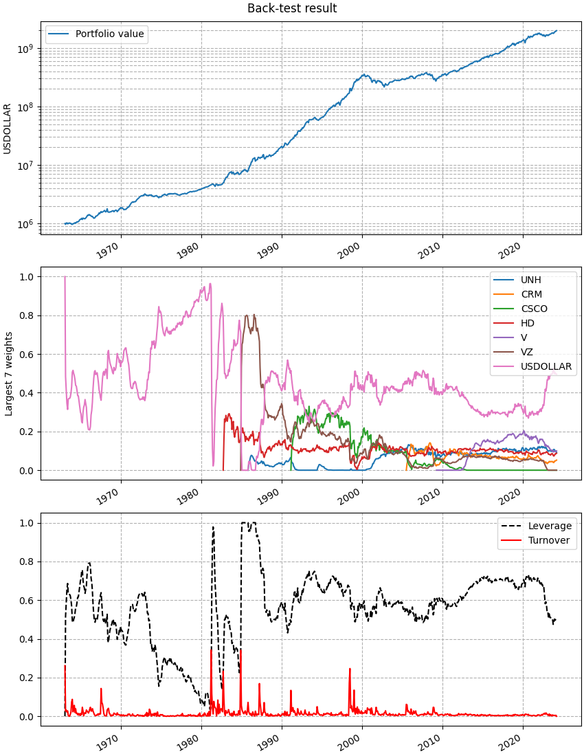
This figure is made by the cvxportfolio.result.BacktestResult.plot() method.#
The result of the cvxportfolio.MultiPeriodOptimization policy
that has the largest out-of-sample growth rate:
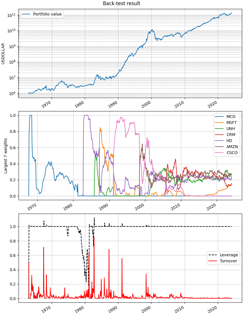
This figure is made by the cvxportfolio.result.BacktestResult.plot() method.#
The result of the cvxportfolio.Uniform policy, which allocates equal
weight to all non-cash assets:
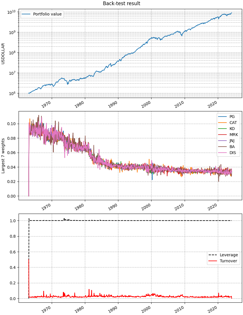
This figure is made by the cvxportfolio.result.BacktestResult.plot() method.#
Finally, the result of the cvxportfolio.MultiPeriodOptimization policy
obtained by automatic hyper-parameter optimization to have largest profit:
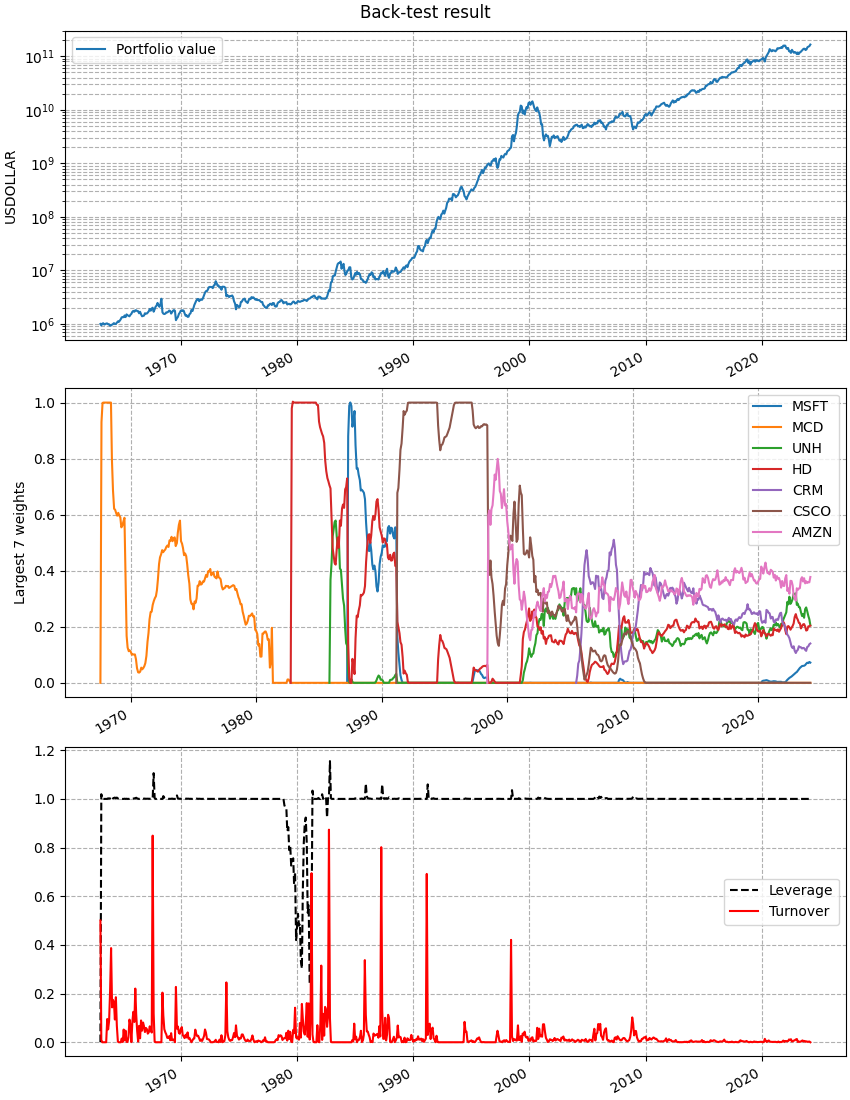
This figure is made by the cvxportfolio.result.BacktestResult.plot() method.#