Wide asset classes ETFs#
ETFs example covering the main asset classes.
This uses an explicit loop to create Multi Period Optimization policies with a grid of values for the risk term multiplier and the transaction cost term multiplier.
All result objects are collected, and then the one with largest Sharpe ratio, and the one with largest growth rate, are shown.
import numpy as np

import cvxportfolio as cvx

UNIVERSE = [
    "QQQ", # nasdaq 100
    "SPY", # US large caps
    'EFA', # EAFE stocks
    "CWB", # convertible bonds
    "IWM", # US small caps
    "EEM", # EM stocks
    "GLD", # Gold
    'TLT', # long duration treasuries
    'HYG', # high yield bonds
    "EMB", # EM bonds (usd)
    'LQD', # investment grade bonds
    'PFF', # preferred stocks
    'VNQ', # US REITs
    'BND', # US total bond market
    'BIL', # US cash
    'TIP', # TIPS
    'DBC', # commodities
    ]

sim = cvx.StockMarketSimulator(UNIVERSE, trading_frequency='monthly')

def make_policy(gamma_trade, gamma_risk):
    """Create policy object given hyper-parameter values.

    :param gamma_trade: Choice of the trading aversion multiplier.
    :type gamma_trade: float
    :param gamma_risk: Choice of the risk aversion multiplier.
    :type gamma_risk: float

    :returns: Policy object with given choices of hyper-parameters.
    :rtype: cvx.policies.Policy instance

    """
    return cvx.MultiPeriodOptimization(cvx.ReturnsForecast()
        - gamma_risk * cvx.FactorModelCovariance(num_factors=10)
        - gamma_trade * cvx.StocksTransactionCost(),
        [cvx.LongOnly(), cvx.LeverageLimit(1)],
        planning_horizon=6, solver='ECOS')

keys = [(gamma_trade, gamma_risk)
    for gamma_trade in np.array(range(10))/10
        for gamma_risk in [.5, 1, 2, 5, 10]]
ress = sim.backtest_many(
    [make_policy(*key) for key in keys], parallel=True)

print('LARGEST SHARPE RATIO')
idx = np.argmax([el.sharpe_ratio for el in ress])

print('gamma_trade and gamma_risk')
print(keys[idx])

print('result')
print(ress[idx])

largest_sharpe_figure = ress[idx].plot()

print('LARGEST GROWTH RATE')
idx = np.argmax([el.growth_rates.mean() for el in ress])

print('gamma_trade and gamma_risk')
print(keys[idx])

print('result')
print(ress[idx])

largest_growth_figure = ress[idx].plot()
This is the output printed to screen when executing this script. You can see many statistics of the back-tests.
Updating data.................
LARGEST SHARPE RATIO
gamma_trade and gamma_risk
(0.9, 10)
result

###########################################################
Universe size                                            18
Initial timestamp                       1994-02-01 14:30:00
Final timestamp                         2024-03-01 14:30:00
Number of periods                                       362
Initial value (USDOLLAR)                          1.000e+06
Final value (USDOLLAR)                            6.180e+06
Profit (USDOLLAR)                                 5.180e+06

Avg. return (annualized)                               6.3%
Volatility (annualized)                                7.2%
Avg. excess return (annualized)                        3.9%
Avg. active return (annualized)                        3.9%
Excess volatility (annualized)                         7.1%
Active volatility (annualized)                         7.1%

Avg. growth rate (annualized)                          6.1%
Avg. excess growth rate (annualized)                   3.6%
Avg. active growth rate (annualized)                   3.6%

Avg. StocksTransactionCost                              0bp
Max. StocksTransactionCost                             40bp
Avg. StocksHoldingCost                                  0bp
Max. StocksHoldingCost                                  0bp

Sharpe ratio                                           0.55
Information ratio                                      0.55

Avg. drawdown                                         -3.7%
Min. drawdown                                        -23.2%
Avg. leverage                                         68.1%
Max. leverage                                        100.4%
Avg. turnover                                          3.3%
Max. turnover                                         93.5%

Avg. policy time                                     0.025s
Avg. simulator time                                  0.007s
    Of which: market data                            0.001s
Total time                                          11.750s
###########################################################

LARGEST GROWTH RATE
gamma_trade and gamma_risk
(0.0, 5)
result

###########################################################
Universe size                                            18
Initial timestamp                       1994-02-01 14:30:00
Final timestamp                         2024-03-01 14:30:00
Number of periods                                       362
Initial value (USDOLLAR)                          1.000e+06
Final value (USDOLLAR)                            9.716e+06
Profit (USDOLLAR)                                 8.716e+06

Avg. return (annualized)                               8.2%
Volatility (annualized)                               11.3%
Avg. excess return (annualized)                        5.8%
Avg. active return (annualized)                        5.8%
Excess volatility (annualized)                        11.3%
Active volatility (annualized)                        11.3%

Avg. growth rate (annualized)                          7.6%
Avg. excess growth rate (annualized)                   5.1%
Avg. active growth rate (annualized)                   5.1%

Avg. StocksTransactionCost                              1bp
Max. StocksTransactionCost                             84bp
Avg. StocksHoldingCost                                  0bp
Max. StocksHoldingCost                                  0bp

Sharpe ratio                                           0.51
Information ratio                                      0.51

Avg. drawdown                                         -6.4%
Min. drawdown                                        -32.7%
Avg. leverage                                         85.6%
Max. leverage                                        100.9%
Avg. turnover                                          4.6%
Max. turnover                                        100.0%

Avg. policy time                                     0.024s
Avg. simulator time                                  0.007s
    Of which: market data                            0.001s
Total time                                          11.316s
###########################################################
And these are the figure that are plotted.
The result of the cvxportfolio.MultiPeriodOptimization policy
that has the largest out-of-sample Sharpe ratio:
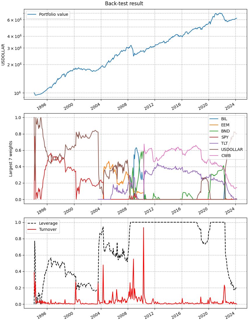
This figure is made by the cvxportfolio.result.BacktestResult.plot() method.#
The result of the cvxportfolio.MultiPeriodOptimization policy
that has the largest out-of-sample growth rate:
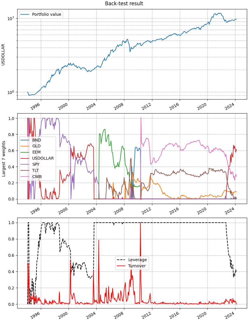
This figure is made by the cvxportfolio.result.BacktestResult.plot() method.#