User-provided forecasters#
Simple example for providing user-defined forecasters to Cvxportfolio.
This example shows how the user can provide custom-made predictors for expected returns and covariances, at each point in time (when used in back-test). These forecasters can be used seamlessly inside a cvxportfolio back-test, or online execution.
Note
No attempt is being made here to find good values of the hyper-parameters; this is simply used to show how to provide custom forecasters.
One interesting feature of this is that Cvxportfolio guarantees that no look-ahead biases are introduced when making these forecasts. The data is sliced so that, at each point in time, only past data is provided to the forecasters.
More advanced custom predictors can be provided as well; the relevant interfaces will be documented in the future. Internally, Cvxportfolio forecasters use something very similar to this, but also have a recursive execution model which enables them to compose objects, are aware of the current trading universe and future (expected) trading calendar (for multi-period applications), and have a destructor which is used for memory safety when parallelizing back-tests. However, this simple interface is guaranteed to work.
You can see the documentation of the
cvxportfolio.estimator.Estimator.values_in_time() method that is used
here for the full list of available arguments.
import cvxportfolio as cvx

# Here we define a class to forecast expected returns
# There is no need to inherit from a base class, in this simple case
class WindowMeanReturns: # pylint: disable=too-few-public-methods
    """Expected return as mean of recent window of past returns.

    This is only meant as an example of how to define a custom forecaster;
    it is not very interesting. Since version ``1.2.0`` a similar
    functionality has been included in the default forecasters classes.

    :param window: Window used for the mean returns.
    :type window: int
    """

    def __init__(self, window=20):
        self.window = window

    def values_in_time(self, past_returns, **kwargs):
        """This method computes the quantity of interest.

        It has many arguments, we only need to use ``past_returns`` in this
        case.

        :param past_returns: Historical market returns for all assets in
            the current trading universe, up to each time at which the
            policy is evaluated.
        :type past_returns: pd.DataFrame
        :param kwargs: Other, unused, arguments to :meth:`values_in_time`.
        :type kwargs: dict

        :returns: Estimated mean returns.
        :rtype: pd.Series

        .. note::

            The last column of ``past_returns`` are the cash returns.
            You need to explicitely skip them otherwise Cvxportfolio will
            throw an error.
        """
        return past_returns.iloc[-self.window:, :-1].mean()

# Here we define a class to forecast covariances
# There is no need to inherit from a base class, in this simple case
class WindowCovariance: # pylint: disable=too-few-public-methods
    """Covariance computed on recent window of past returns.

    This is only meant as an example of how to define a custom forecaster;
    it is not very interesting. Since version ``1.2.0`` a similar
    functionality has been included in the default forecasters classes.

    :param window: Window used for the covariance computation.
    :type window: int
    """

    def __init__(self, window=20):
        self.window = window

    def values_in_time(self, past_returns, **kwargs):
        """This method computes the quantity of interest.

        It has many arguments, we only need to use ``past_returns`` in this
        case.

        :param past_returns: Historical market returns for all assets in
            the current trading universe, up to each time at which the
            policy is evaluated.
        :type past_returns: pd.DataFrame
        :param kwargs: Other, unused, arguments to :meth:`values_in_time`.
        :type kwargs: dict

        :returns: Estimated covariance.
        :rtype: pd.DataFrame

        .. note::

            The last column of ``past_returns`` are the cash returns.
            You need to explicitely skip them otherwise Cvxportfolio will
            throw an error.
        """
        return past_returns.iloc[-self.window:, :-1].cov()

# define the hyper-parameters
WINDOWMU = 252
WINDOWSIGMA = 252
GAMMA_RISK = 5
GAMMA_TRADE = 3

# define the forecasters
mean_return_forecaster = WindowMeanReturns(WINDOWMU)
covariance_forecaster = WindowCovariance(WINDOWSIGMA)

# define the policy
policy = cvx.SinglePeriodOptimization(
    objective = cvx.ReturnsForecast(r_hat = mean_return_forecaster)
        - GAMMA_RISK * cvx.FullCovariance(Sigma = covariance_forecaster)
        - GAMMA_TRADE * cvx.StocksTransactionCost(),
    constraints = [cvx.LongOnly(), cvx.LeverageLimit(1)]
    )

# define the simulator
simulator = cvx.StockMarketSimulator(['AAPL', 'GOOG', 'MSFT', 'AMZN'])

# back-test
result = simulator.backtest(policy, start_time='2020-01-01')

# show the result
print(result)
figure = result.plot()
This is the output printed to screen when executing this script. If you compare to a back-test using the standard Cvxportfolio forecasters you may notice that the default have faster execution time (that’s shown in the policy times). That is because Cvxportfolio built-in forecasters are optimized for sequential evaluation, at each point in time of a back-test they don’t necessarily compute the forecasts from scratch, but update the ones computed at the period before (if possible).
Updating data....

#################################################################
Universe size                                                   5
Initial timestamp                       2020-01-02 14:30:00+00:00
Final timestamp                         2024-04-05 13:30:00+00:00
Number of periods                                            1072
Initial value (USDOLLAR)                                1.000e+06
Final value (USDOLLAR)                                  1.471e+06
Profit (USDOLLAR)                                       4.710e+05

Avg. return (annualized)                                    10.7%
Volatility (annualized)                                     18.0%
Avg. excess return (annualized)                              8.7%
Avg. active return (annualized)                              8.7%
Excess volatility (annualized)                              18.0%
Active volatility (annualized)                              18.0%

Avg. growth rate (annualized)                                9.1%
Avg. excess growth rate (annualized)                         7.1%
Avg. active growth rate (annualized)                         7.1%

Avg. StocksTransactionCost                                    0bp
Max. StocksTransactionCost                                    2bp
Avg. StocksHoldingCost                                        0bp
Max. StocksHoldingCost                                        0bp

Sharpe ratio                                                 0.49
Information ratio                                            0.49

Avg. drawdown                                              -10.8%
Min. drawdown                                              -23.7%
Avg. leverage                                               49.5%
Max. leverage                                              100.0%
Avg. turnover                                                0.5%
Max. turnover                                               50.0%

Avg. policy time                                           0.003s
Avg. simulator time                                        0.003s
    Of which: market data                                  0.001s
    Of which: result                                       0.000s
Total time                                                 6.403s
#################################################################
And this is the figure that is plotted. You can see that, compared to the standard Cvxportfolio forecasts (which use all available historical data at each point in time) this back-test has a much less stable allocation, and changes much more with the market conditions.
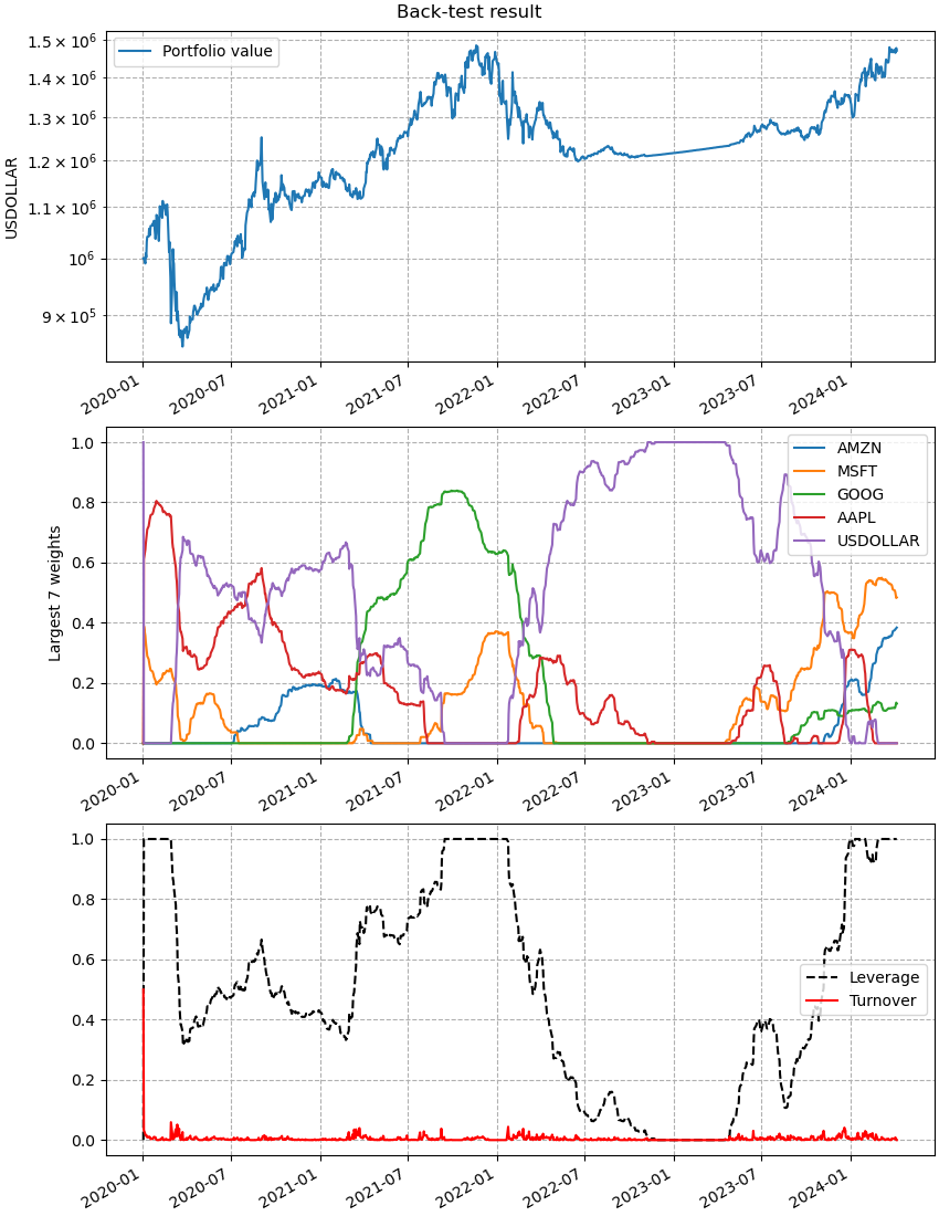
This figure is made by the cvxportfolio.result.BacktestResult.plot() method.#